Histogram Maker

What is a Histogram?

A histogram is a statistical chart that displays the frequency distribution of a continuous dataset. Unlike a bar chart which compares discrete, separate categories, a histogram groups numerical data into adjacent intervals called bins (or class intervals). The height of each bar represents the count (frequency) of values that fall within that range, giving you an immediate visual summary of how your data is distributed.

Histograms are one of the most fundamental tools in exploratory data analysis (EDA). They reveal the underlying shape of a distribution whether it is symmetric, skewed left or right, bimodal, or uniform and help analysts spot outliers, clusters, and gaps that raw numbers alone cannot convey. Our free online histogram maker handles all the calculations automatically, letting you focus on interpreting the story your data tells.

When to Use a Histogram

• Visualizing the distribution shape of test scores, measurements, or survey responses
• Identifying whether data follows a normal (bell-curve) distribution
• Detecting outliers and gaps in a dataset
• Analyzing process performance in quality control (e.g., product dimensions)
• Summarizing large datasets like hundreds or thousands of values into a readable chart
• Comparing frequency distributions before and after a change

Histogram vs Bar Chart — Key Difference

This is the most common point of confusion. A bar chart compares distinct categories (apples vs oranges, Q1 vs Q2) with gaps between the bars. A histogram displays a continuous numerical range with no gaps — the touching bars visually communicate that the data flows from one interval directly into the next. If you have categories, use our bar graph maker. If you have a column of numbers you want to understand the spread of, a histogram is the right tool.

How Bin Count Affects Your Histogram

The most important decision in creating a histogram is choosing the number of bins. Too few bins and you lose detail because the entire distribution compresses into two or three large bars. Too many bins and you get noise as every value gets its own bar and the shape becomes impossible to read.

Our histogram graph generator offers four methods so you always get an appropriate starting point:

• Sturges' Rule (default): bins = ⌈log₂(n) + 1⌉. Works best for roughly normal distributions with up to a few hundred data points. The most widely taught formula in introductory statistics.
• Square Root Rule: bins = ⌈√n⌉. A simple, conservative rule that avoids over-smoothing. Useful when data is uniformly distributed.
• Rice Rule: bins = ⌈2 · n^(1/3)⌉. A middle-ground formula that tends to produce slightly more bins than Sturges' for larger datasets.
• Custom: enter any number of bins between 2 and 100. Use this when you have domain knowledge about meaningful class intervals (e.g., age groups in 5-year bands).

After generating your chart, try adjusting the bin count up and down to see which setting reveals the most useful pattern in your data.

Key Features of Our Free Histogram Maker

Flexible Data Input

• Upload Excel (.xlsx, .xls) or CSV files with header rows detected and skipped automatically
• Paste a column of numbers directly from Excel or Google Sheets with Ctrl+V
• Enter values manually in the single-column data table
• Supports any numeric format including decimals and negatives

Live Descriptive Statistics

Every time you generate a histogram, a statistics panel updates instantly showing count, mean, median, standard deviation, minimum, and maximum for your dataset. This removes the need to open a spreadsheet separately as the core descriptive statistics are right next to the chart.

Full Visual Control

• 4 auto-binning methods plus manual bin count (2–100 bins)
• Custom X-axis range to focus on a specific data window
• 7 color presets with individual fill and border color pickers
• Bar opacity and border width sliders for fine-tuned styling
• Optional frequency labels on each bar
• Probability Density mode which normalizes the Y-axis to show relative density instead of raw counts, useful for comparing distributions of different sizes
• Chart title and axis labels that appear on all exported files

Three Export Formats

• PNG: high-resolution with transparent background, perfect for reports and slides
• JPEG: smaller file size for presentations and web use
• SVG: true scalable vector export with bars, axes, gridlines, and labels — not a screenshot of the canvas

How to Make a Histogram Online — Step by Step

Histogram Maker for Excel Users

Excel's built-in histogram tool requires enabling the Analysis ToolPak add-in, configuring bin ranges manually in a separate column, and re-running the tool every time your data changes. Our histogram maker for Excel users is simpler: copy your data column (including any header row and the tool auto-detects and skips it), paste it directly into the data table, and your histogram is ready in one click. No add-ins, no bin configuration tables, no re-running. If you need the chart in Excel afterward, download the PNG or SVG and insert it as an image.

Understanding Distribution Shapes

Once you have your histogram, here is how to read what the shape is telling you:

• Bell curve (normal distribution): symmetric, single peak in the center. Common in natural measurements like height or test scores. Mean ≈ median ≈ mode.
• Right-skewed (positively skewed): long tail on the right, most values clustered on the left. Common in income data, time-to-failure data. Mean > median.
• Left-skewed (negatively skewed): long tail on the left. Common in age-at-retirement data. Mean < median.
• Bimodal: two distinct peaks. Often signals two different groups mixed in one dataset (e.g., exam scores for two classes combined).
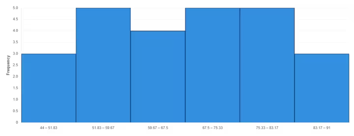
• Uniform: all bins roughly equal height. Suggests values are spread evenly across the range, possibly from a random or flat distribution.
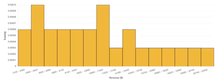
• Right-heavy with outlier spike: most bars short, one bar much taller at the extreme. Inspect those values; they may be data entry errors or legitimate anomalies.

Probability Density Histograms

When comparing two datasets of different sizes, raw frequency counts are misleading because the larger dataset will always look taller. Enabling Probability Density mode in our tool normalizes the Y-axis so that the total area of all bars equals 1. This lets you compare the shape of distributions directly, regardless of sample size. It is the format used in academic publications and statistical software like R and Python's matplotlib.

Our Other Statistical and Data Visualization Tools

Ready to Visualize Your Distribution?

Whether you are a student analysing survey responses, a data analyst checking normality assumptions, or a quality engineer reviewing process measurements, our free online histogram maker delivers publication-ready charts in under a minute. Enter your data above and generate your first histogram with no sign-up, no watermarks, and no limits.

Explore our full suite of free data visualization tools.